 David Keyes
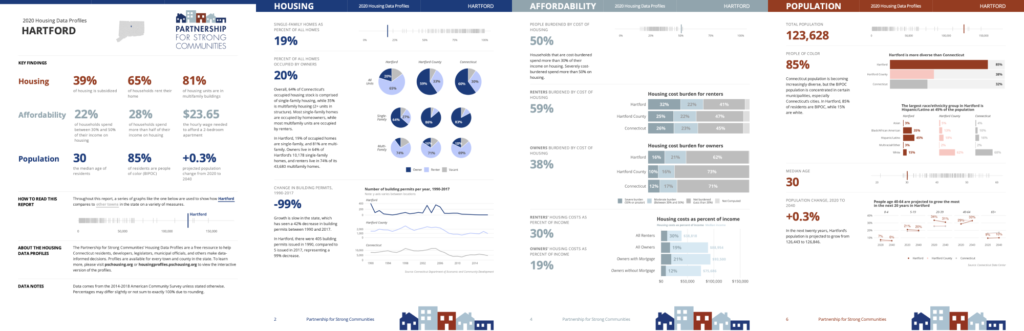
In a lot of the consulting work that R for the Rest of Us does, we do complex layouts of the sort are typically done with page layout software like Adobe InDesign. For example, in the reports we did on demographic and housing data in Connecticut, the charts were laid out in a complex grid across multiple pages.
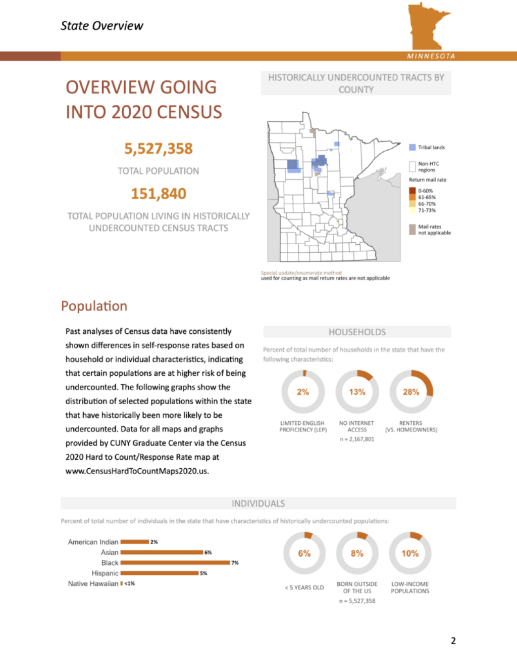
Or take a look at these reports, done in partnership with the Democracy Funders Collaborative's Census Subgroup and ORS Impact, that provide an overview of efforts to promote the 2020 Census across the United States.
I'm often asked how we did these layouts. The truth is, it can be a bit complicated, and the answer varies depending on a number of factors. But, when an R in 3 Months participant asked this same question recently, I knew I had to come up with an answer to share.
Fortunately for me, I work with the very talented Charlie Hadley, who makes detailed videos explaining complex concepts to R learners. I asked Charlie to put together on some tips on the topic and she made some great videos showing how to make multicolumn layouts in RMarkdown. Here they are.
Option #1: Use patchwork or cowplot to combine multiple ggplot2 plots
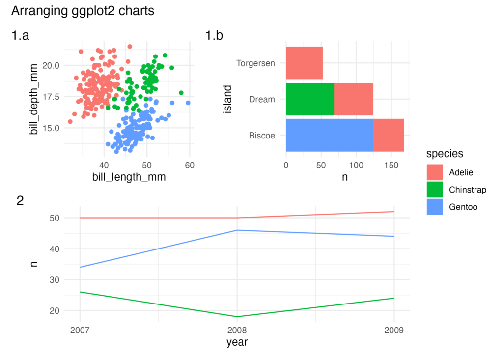
There are two packages, patchwork and cowplot, that allow you to put multiple plots together. You can use this technique to make a multicolumn layout, as in this example:
Watch the video below as Charlie explains how this was made and follow her code below that.
---
title: "Two column ggplot2 charts"
output: html_document
---

```{r setup, include=FALSE}
knitr::opts_chunk$set(
	echo = TRUE,
	message = FALSE,
	warning = FALSE
)
library(tidyverse)
library(patchwork)
library(cowplot)
library(palmerpenguins)
```

```{r original_charts, include=FALSE}
gg_penguin_scatter <- penguins %>%
  ggplot(aes(x = bill_length_mm,
             y = bill_depth_mm,
             color = species)) +
  geom_point()
gg_penguin_bar_chart <- penguins %>%
  count(island, species) %>%
  ggplot(aes(x = n,
             y = island,
             fill = species)) +
  geom_col()
gg_penguins_timeline <- penguins %>%
  count(year, species) %>%
  ggplot(aes(x = year,
             y = n,
             color = species)) +
  geom_line() +
  scale_x_continuous(n.breaks = 3)
```


# Intro

Often you'll want to arrange multiple {ggplot2} charts together with tags and titles, eg:

```{r echo=FALSE}
ptchw_chart <- ( ( gg_penguin_scatter | gg_penguin_bar_chart ) + plot_layout(tag_level = 'new') ) / gg_penguins_timeline + plot_layout(guides = 'collect')
gg_ptch_chart <- ptchw_chart &
  guides(color = guide_none()) &
  plot_annotation(tag_levels = c('1', 'a'), tag_sep = ".") &
  plot_annotation(title = "Arranging ggplot2 charts") &
  theme_minimal()
ggsave("gg_ptch_chart.png",
       gg_ptch_chart)
gg_ptch_chart
```

There are two different packages you can choose from, {cowplot} and {patchwork}. They are both very popular in the R community and it's almost down to personal choice which one you prefer. I've tried to differentiate them a little bit:

- {cowplot}

  - Charts are explicitly built within a grid using `plot_grid()`. The layout is controlled by specifying the number of rows and columns in the chart

  - Nested `plot_grid()` are required to get a single chart to span multiple rows or columns.

  - Themes need to be applied to individual charts.

  - Legends need to be extracted from charts and manually placed within a `plot_grid()`.

> {cowplot} allows extreme precision over your charts. Complex collections of charts with inset charts and custom looking legends can be created.


- {patchwork}

  - Charts are built using `(p1 + p2) / p3` syntax, `p3` will be placed under `p1` and `p2`.

  - Because there is no grid system `p3` will automatically span the entire width of the chart.

  - Themes can be applied to the entire patchwork chart.

  - Legends can be automatically collected.

> {patchwork} feels and behaves like a ggplot2 extension, a lot of things are automated. It can become painful to create extremely customised charts.

## cowplot

We need to create a nested plot_grid() for the timeline chart to span the width of the chart:


```{r}
plot_grid(plot_grid(gg_penguin_scatter, gg_penguin_bar_chart),
          plot_grid(gg_penguins_timeline),
          nrow = 2)
```

In the chart below our goal is to collect together the legends and change the theme:

- The legend is extracted from the bar chart with `get_legend()`

- The legends for all charts are disabled with `theme(legend.position = "none")`

- The legend is attached to the chart using another `plot_grid()`

- The theme has to be changed for all individual charts.

```{r}
cwp_legend <- get_legend(gg_penguin_bar_chart)
cwp_collected <-
  plot_grid(
    plot_grid(
      gg_penguin_scatter + theme_minimal() + theme(legend.position = "none"),
      gg_penguin_bar_chart + theme_minimal() + theme(legend.position = "none")
    ),
    plot_grid(gg_penguins_timeline + theme_minimal() + theme(legend.position = "none")),
    nrow = 2
  )
plot_grid(
  cwp_collected,
  cwp_legend,
  ncol = 2,
  rel_widths = c(8, 1)
)
```

Automatic labelling only works within an individual `plot_grid()`. We therefore need to add manual labels into the chart:

```{r}
cwp_labelled <-
  plot_grid(
    plot_grid(
      gg_penguin_scatter + theme_minimal() + theme(legend.position = "none"),
      gg_penguin_bar_chart + theme_minimal() + theme(legend.position = "none"),
      labels = c("1.a", "1.b")
    ),
    plot_grid(gg_penguins_timeline + theme_minimal() + theme(legend.position = "none"),
              labels = "2"),
    nrow = 2
  )
plot_grid(
  cwp_labelled,
  cwp_legend,
  ncol = 2,
  rel_widths = c(8, 1)
)
```


## Patchwork

Our basic layout is achieved as follows

```{r}
(gg_penguin_scatter + gg_penguin_bar_chart ) / gg_penguins_timeline
```

To change the theme of all subplots we use `&`

```{r}
ptwc_basic <- (gg_penguin_scatter + gg_penguin_bar_chart ) / gg_penguins_timeline
ptwc_basic & theme_minimal()
```

To collect together the legends we go through two steps:

- Remove the guides for the `color` aesthetic, leaving only the fill guide.

- Use `plot_layout(guides = "collect")` to collect the remaining guides together

```{r}
ptchw_collected <- ( gg_penguin_scatter | gg_penguin_bar_chart ) / gg_penguins_timeline + plot_layout(guides = "collect")
ptchw_collected &
  guides(color = guide_none()) &
  theme_minimal()
```

{patchwork} can do automatic tagging, the documentation shows the different systems of counting available.

```{r}
ptchw_auto_tagging <- ( ( gg_penguin_scatter | gg_penguin_bar_chart ) + plot_layout(tag_level = 'new') ) / gg_penguins_timeline + plot_layout(guides = "collect")
ptchw_auto_tagging &
  guides(color = guide_none()) &
  plot_annotation(tag_levels = c('1', 'a'), tag_sep = ".") &
  theme_minimal()
```

Manual tagging

```{r}
ptchw_manual_tagging <- ( gg_penguin_scatter + labs(tag = "scatter") | gg_penguin_bar_chart + labs(tag = "bar") ) / gg_penguins_timeline + labs(tag = "line") + plot_layout(guides = "collect")
ptchw_manual_tagging &
  guides(color = guide_none()) &
  theme_minimal()
```
Option #2: Use custom CSS in HTML files
If you're knitting your RMarkdown documents to HTML reports, you'll need to use custom CSS to add columns. You can do this using what's known as flexbox or bootstrap.
The video below demonstrates the differences between these two approaches (code follows):
---
title: "Two Columns: html_document"
output: html_document
---

```{r setup, include=FALSE}
knitr::opts_chunk$set(echo = TRUE)
```

# Intro

There are two web frameworks available to us for creating multiple columns in html_document .Rmd files

- [**flexbox**](https://css-tricks.com/snippets/css/a-guide-to-flexbox/):

  - Very flexible solution for controlling a single row of content

  - Disadvantage: flexbox columns don't reflow based on browser width, so may be difficult to read on mobile devices.

  - Advantage: flexbox columns don't reflow, making them a very good choice


extremely flexible solution for reflowing content, it does not automatically scale to the width of the browser window.


- [**bootstrap**](https://getbootstrap.com/): designed to reflow content according to the browser width by default.

You could use either framework to achieve the same layouts, but they would require different code for each and some things might be easier in one than the other. To give you **practical** solutions I'm going to show you how to do two different things:

- Content in two columns **independent of browser width** using flexbox

- Content that reflows to one column when the browser becomes narrow using bootstrap

## HTML & `<div>` elements

Web pages are written in HTML. HTML is composed of open and close tags, for instance this is how we would create a heading and subheading with the h1 and h2 tags

```{html}
<h1>Heading</h1>
<h2>Sub heading</h2>
```

The `<div>` tag allows us to split up components of a web page. In this document we're using <div> to define a row than then contains two <div> components, one for each column.

In RMarkdown we have the choice between typing out <div> tags or using pairs of `:::`. Because [lots of documentation](https://bookdown.org/yihui/rmarkdown-cookbook/multi-column.html) uses the `:::` approach I've provided examples of both syntaxes.


# Two columns independent of browser width

This uses **flexbox**

## Using :::

:::: {style="display: flex;"}

::: {}

This is the first column (on the left)

```{r}
str(quakes)
```

:::

::: {}

... and this is the second column (on the right)

```{r}
str(chickwts)
```

:::

::::

## Using `<div>`

<div style="display: flex;">

<div>

This is the first column (on the left)

```{r}
str(quakes)
```

</div>

<div>

... and this is the second column (on the right)

```{r}
str(chickwts)
```

</div>

</div>


# Two columns dependent on browser width

This uses **bootstrap**.

## Using `:::`

:::: {class='fluid-row'}

::: {class='col-md-6'}

1st column when browser is wide

```{r}
head(datasets::airmiles)
```

:::

::: {class='col-md-6'}

... 2nd column when browser is wide

```{r}
head(datasets::AirPassengers)
```

:::

::::

## Using `<div>`

<div class='fluid-row'>

<div class='col-md-6'>

1st column when browser is wide

```{r}
head(datasets::airmiles)
```

</div>

<div class='col-md-6'>

... 2nd column when browser is wide

```{r}
head(datasets::AirPassengers)
```

</div>

</div>
While HTML as an export format is common, many people work in organizations that want PDFs. Fortunately, the pagedown package (and Thomas Vroylandt and my pagedreport package) actually create HTML documents that they the convert to PDFs. As a result, you can use CSS to create multicolumn layouts in pagedown, as Charlie demonstrates:
---
title: "Pagedown"
output:
  pagedown::html_letter:
    self_contained: false
links-to-footnotes: true
paged-footnotes: true
---

```{r setup, include=FALSE}
knitr::opts_chunk$set(
	echo = FALSE,
	message = FALSE,
	warning = FALSE
)
library(tidyverse)
library(palmerpenguins)
```

::: from
Charlie Joey Hadley
Bristol
United Kingdom
Email: charlie@rfortherestofus.com
:::

# Intro

[{pagedown}](https://github.com/rstudio/pagedown) is designed to solve an annoying problem in RMarkdown

> Formatting PDF RMarkdown documents is difficult and requires LaTeX.

The {pagedown} solution is to allow us to write HTML documents with pagination (and printing) as the primary goal. It's really very good at it:

- pagedown::thesis_paged

- pagedown::jss_paged

- pagedown::html_resume

- pagedown::poster_relaxed

- pagedown::business_card

The **best** choice for creating multiple columns in {pagedown} is flexbox because it's browser width agnostic.

As before, we can use either `<div>` tags or `:::`

## Using ::: {.page-break-before}

:::: {style="display: flex;"}

::: {}

This is the first column (on the left)

```{r}
penguins %>%
  ggplot(aes(x = bill_length_mm,
             y = bill_depth_mm,
             color = species)) +
  geom_point()
```

:::

::: {}

... and this is the second column (on the right)

```{r}
penguins %>%
  ggplot(aes(x = bill_length_mm,
             y = bill_depth_mm,
             color = island)) +
  geom_point()
```

:::

::::

## Using `<div>`

<div style="display: flex;">

<div>

This is the first column (on the left)

```{r}
penguins %>%
  ggplot(aes(x = bill_length_mm,
             y = bill_depth_mm,
             color = species)) +
  geom_point()
```

</div>

<div>

... and this is the second column (on the right)

```{r}
penguins %>%
  ggplot(aes(x = bill_length_mm,
             y = bill_depth_mm,
             color = island)) +
  geom_point()
```

</div>

</div>
Option #3: Use officedown and officer for multicolumn Word documents
If you need to export your RMarkdown document to Word, custom CSS won’t work. You can, of course, use option #1 to create multicolumn plots and then put those into Word. Another approach for Word documents is to use the officedown and officer packages. Together, these two packages allow you to build rich Word documents directly from RMarkdown. This video shows how to create two columnsusing output: officedown::rdocx_document.
---
title: "Two columns in Word Documents"
output: officedown::rdocx_document
---
```{r setup, include=FALSE}
knitr::opts_chunk$set(
echo = TRUE,
message = FALSE,
warning = FALSE
)
library(officer)
library(tidyverse)
library(palmerpenguins)
```
# Intro
There are a collection of packages called [{officeverse}](https://ardata-fr.github.io/officeverse/) for creating and manipulating MS Word and MS Powerpoint documents. To create two column layouts we need to use two of these packages:
- {officedown}: This package provides additional RMarkdown output formats for creating .docx and .pptx files. We change the YAML header to contain `output: officedown::rdocx_document`.
- {officer}: This package allows us to programmatically generate (and modify existing) .docx and .pptx files. We use this package to add column breaks with the `run_columnbreak()` function.
There are two steps to creating multiple columns:
1. Use a pair of HTML comments as follows:
<code>
<!--BLOCK_MULTICOL_START--->
<!---BLOCK_MULTICOL_START--->
</code>
1. Call `run_columnbreak()` as an inline expression at the beginning of the content for the second column.
## What's an inline expression?
An inline R expression allows us to run R code within a Markdown content instead of in a code chunk. It looks like this:
```{yaml}
There are `r 2+2` lights
```
## Page break
I've manually inserted a page break here with `run_pagebreak()`
```{r}
run_pagebreak()
```
# Example two column layout
The two column content begins underneath the HTML comment. Remember that the HTML comment won't display inside the output document.
<!---BLOCK_MULTICOL_START--->
This is the beginning of the first column
```{r echo=FALSE, fig.cap="Penguin scatter plot", fig.cap.style = "Image Caption", fig.width=3, fig.height=3, dpi=300}
gg_penguin_scatter <- penguins %>%
ggplot(aes(x = bill_length_mm,
y = bill_depth_mm,
color = species)) +
geom_point() +
theme_minimal(base_size = 8)
ggsave("gg_penguin_scatter.png",
gg_penguin_scatter,
width = 3,
height = 3,
unit = "in",
dpi = 300)
knitr::include_graphics("gg_penguin_scatter.png")
```
`r run_columnbreak()`This sentence begins the second column.
```{r echo=FALSE, fig.cap="Penguin scatter plot", fig.cap.style = "Image Caption", fig.width=3, fig.height=3, dpi=300}
gg_penguin_bar <- penguins %>%
count(island, species) %>%
ggplot(aes(x = n,
y = island,
fill = species)) +
geom_col() +
theme_minimal(base_size = 8)
ggsave("gg_penguin_bar.png",
gg_penguin_bar,
width = 3,
height = 3,
unit = "in",
dpi = 300)
knitr::include_graphics("gg_penguin_bar.png")
```
The multi column will end after this sentence.
<!---BLOCK_MULTICOL_STOP--->
**This text** is just below the HTML comment so Word continues in single column mode. There's another manual page break here.
```{r}
run_pagebreak()
```
# Customising column appearance
By modifying the closing HTML comment it's possible to customise the appearance of the columns:
<!---BLOCK_MULTICOL_START--->
This is the beginning of the first column
```{r echo=FALSE, fig.cap="Penguin scatter plot", fig.cap.style = "Image Caption", fig.width=3, fig.height=3, dpi=300}
gg_penguin_scatter <- penguins %>%
ggplot(aes(x = bill_length_mm,
y = bill_depth_mm,
color = species)) +
geom_point() +
theme_minimal(base_size = 8)
ggsave("gg_penguin_scatter.png",
gg_penguin_scatter,
width = 3,
height = 3,
unit = "in",
dpi = 300)
knitr::include_graphics("gg_penguin_scatter.png")
```
`r run_columnbreak()`This sentence begins the second column.
```{r echo=FALSE, fig.cap="Penguin scatter plot", fig.cap.style = "Image Caption", fig.width=3, fig.height=3, dpi=300}
gg_penguin_bar <- penguins %>%
count(island, species) %>%
ggplot(aes(x = n,
y = island,
fill = species)) +
geom_col() +
theme_minimal(base_size = 8)
ggsave("gg_penguin_bar.png",
gg_penguin_bar,
width = 3,
height = 3,
unit = "in",
dpi = 300)
knitr::include_graphics("gg_penguin_bar.png")
```
The multi column will end after this sentence.
<!---BLOCK_MULTICOL_STOP{widths: [3,3], space: 0.2, sep: true}--->Creating multicolumn layouts may seem like a small thing, but it can have a huge impact. Since the R for the Rest of Us team started using the techniques above, we've been able to create reports from start to finish in R. No longer do we need to bring in a graphic designer to do the final layout. It's a huge timesaver and also makes it possible to do things like automatically make 170+ reports.
You need to be signed-in to comment on this post. Login.
Jean Hong
May 23, 2023
Thank you for posting these options in creating a multicolumn layout. The third option using officer and officedown worked as expected. The only issue is that when knitting (and rendering the parameterized reports) the headers and footers aren't showing up as they did prior to inserting the multicolumn layout sections.
Before inserting the multicolumn layout sections, the headers and footers would be across all pages of the knitted document (via the reference doc). However, after inserting the multicolumn layout sections, the headers and footers from the reference doc are only showing up in the last word section (after all the multicolumn formatting). Any advice on how to get the headers and footers to be continuous across the entire word doc?