Create a Custom Theme

This lesson is called Create a Custom Theme, part of the Going Deeper with R course. This lesson is called Create a Custom Theme, part of the Going Deeper with R course.

Transcript

Click on the transcript to go to that point in the video. Please note that transcripts are auto generated and may contain minor inaccuracies.

View code shown in video

# Load Packages -----------------------------------------------------------

library(tidyverse)
library(fs)
library(scales)
library(ggrepel)
library(ggtext)

# Create Directory --------------------------------------------------------

dir_create("data")

# Download Data -----------------------------------------------------------

# download.file("https://github.com/rfortherestofus/going-deeper-v2/raw/main/data/third_grade_math_proficiency.rds",
#               mode = "wb",
#               destfile = "data/third_grade_math_proficiency.rds")

# Import Data -------------------------------------------------------------

third_grade_math_proficiency <- 
  read_rds("data/third_grade_math_proficiency.rds") |> 
  select(academic_year, school, school_id, district, proficiency_level, number_of_students) |> 
  mutate(is_proficient = case_when(
    proficiency_level >= 3 ~ TRUE,
    .default = FALSE
  )) |> 
  group_by(academic_year, school, district, school_id, is_proficient) |> 
  summarize(number_of_students = sum(number_of_students, na.rm = TRUE)) |> 
  ungroup() |> 
  group_by(academic_year, school, district, school_id) |> 
  mutate(percent_proficient = number_of_students / sum(number_of_students, na.rm = TRUE)) |> 
  ungroup() |> 
  filter(is_proficient == TRUE) |> 
  select(academic_year, school, district, percent_proficient) |> 
  rename(year = academic_year) |> 
  mutate(percent_proficient = case_when(
    is.nan(percent_proficient) ~ NA,
    .default = percent_proficient
  )) |> 
  mutate(percent_proficient_formatted = percent(percent_proficient,
                                                accuracy = 1))


# Theme -------------------------------------------------------------------

theme_dk <- function() {
  
  theme_minimal() +
    theme(axis.title = element_blank(),
          plot.title = element_markdown(),
          plot.title.position = "plot",
          panel.grid = element_blank(),
          axis.text = element_text(color = "grey60",
                                   size = 10),
          legend.position = "none")
  
}

# Plot --------------------------------------------------------------------

top_growth_school <- 
  third_grade_math_proficiency |>
  filter(district == "Portland SD 1J") |> 
  group_by(school) |> 
  mutate(growth_from_previous_year = percent_proficient - lag(percent_proficient)) |> 
  ungroup() |> 
  drop_na(growth_from_previous_year) |>
  slice_max(order_by = growth_from_previous_year,
            n = 1) |> 
  pull(school)

third_grade_math_proficiency |>
  filter(district == "Portland SD 1J") |>
  mutate(highlight_school = case_when(
    school == top_growth_school ~ "Y",
    .default = "N"
  )) |> 
  mutate(percent_proficient_formatted = case_when(
    highlight_school == "Y" & year == "2021-2022" ~ str_glue("{percent_proficient_formatted} of students
                                                             were proficient
                                                             in {year}"),
    highlight_school == "Y" & year == "2018-2019" ~ percent_proficient_formatted,
    .default = NA
  )) |> 
  mutate(school = fct_relevel(school, top_growth_school, after = Inf)) |>
  ggplot(aes(x = year,
             y = percent_proficient,
             group = school,
             color = highlight_school,
             label = percent_proficient_formatted)) +
  geom_line() +
  geom_text_repel(hjust = 0,
                  lineheight = 0.9,
                  direction = "x") +
  scale_color_manual(values = c(
    "N" = "grey90",
    "Y" = "orange"
  )) +
  scale_y_continuous(labels = percent_format()) +
  scale_x_discrete(expand = expansion(add = c(0.05, 0.5))) +
  annotate(geom = "text",
           x = 2.02,
           y = 0.6,
           hjust = 0,
           lineheight = 0.9,
           color = "grey70",
           label = str_glue("Each grey line
                            represents one school")) +
  labs(title = str_glue("<b style='color: orange;'>{top_growth_school}</b> showed large growth in math proficiency over the last two years")) +
  theme_dk()

Your Turn

Solution

How you create your theme is up to you! Here is an example of me creating a theme called theme_student().

# Load Packages -----------------------------------------------------------

library(tidyverse)
library(fs)
library(scales)
library(ggrepel)
library(ggtext)

# Create Directory --------------------------------------------------------

dir_create("data")

# Download Data -----------------------------------------------------------

# download.file("https://github.com/rfortherestofus/going-deeper-v2/raw/main/data/enrollment_by_race_ethnicity.rds",
#               mode = "wb",
#               destfile = "data/enrollment_by_race_ethnicity.rds")

# Import Data -------------------------------------------------------------

enrollment_by_race_ethnicity <-
  read_rds("data/enrollment_by_race_ethnicity.rds") |> 
  select(-district_institution_id)  |> 
  select(year, district, everything()) |> 
  mutate(year = case_when(
    year == "School 2021-22" ~ "2021-2022",
    year == "School 2022-23" ~ "2022-2023",
  )) |> 
  mutate(pct_formatted = percent(pct, 
                                 accuracy = 1))


# Theme -------------------------------------------------------------------

theme_student <- function() {
  
  theme_minimal() +
    theme(axis.title = element_blank(),
          plot.title = element_markdown(),
          plot.title.position = "plot",
          panel.grid = element_blank(),
          axis.text = element_text(color = "grey60",
                                   size = 10),
          legend.position = "none")
  
}

# Plot --------------------------------------------------------------------

top_growth_district <- 
  enrollment_by_race_ethnicity |> 
  filter(race_ethnicity == "Hispanic/Latino") |> 
  group_by(district) |> 
  mutate(growth_from_previous_year = pct - lag(pct)) |> 
  ungroup() |> 
  drop_na(growth_from_previous_year) |>
  slice_max(order_by = growth_from_previous_year,
            n = 1) |> 
  pull(district)

enrollment_by_race_ethnicity |> 
  filter(race_ethnicity == "Hispanic/Latino") |> 
  mutate(highlight_district = case_when(
    district == top_growth_district ~ "Y",
    .default = "N"
  )) |> 
  mutate(pct_formatted = case_when(
    highlight_district == "Y" & year == "2022-2023" ~ str_glue("{pct_formatted} of students
                                                               were Hispanic/Latino
                                                               in {year}"),
    highlight_district == "Y" & year == "2021-2022" ~ pct_formatted,
    .default = NA
  )) |>
  mutate(district = fct_relevel(district, top_growth_district, after = Inf)) |>
  ggplot(aes(x = year, 
             y = pct,
             group = district,
             color = highlight_district,
             label = pct_formatted)) +
  geom_line() +
  geom_text_repel(hjust = 0,
                  lineheight = 0.9,
                  direction = "x") +
  scale_color_manual(values = c(
    "N" = "grey90",
    "Y" = "orange"
  )) +
  scale_y_continuous(labels = percent_format()) +
  scale_x_discrete(expand = expansion(add = c(0.05, 0.5))) +
  annotate(geom = "text",
           x = 2.02,
           y = 0.4,
           hjust = 0,
           lineheight = 0.9,
           color = "grey70",
           label = str_glue("Each grey line
                            represents one district")) +
  labs(title = str_glue("<b style='color: orange;'>{top_growth_district}</b> saw a large growth in its Hispanic/Latino student population over the last two years")) +
  theme_student()

Make your own custom theme and apply it to your plot.
If you want to confirm that it works with other plots, copy it to another project and try it there.

Learn More

If you want to see a bunch of complete themes ready for your use, I've written a blog post that may be of interest to you. If you want to dive deep on creating custom themes, Andrew Heiss has some great materials here. This talk by Cara Thompson is also great.

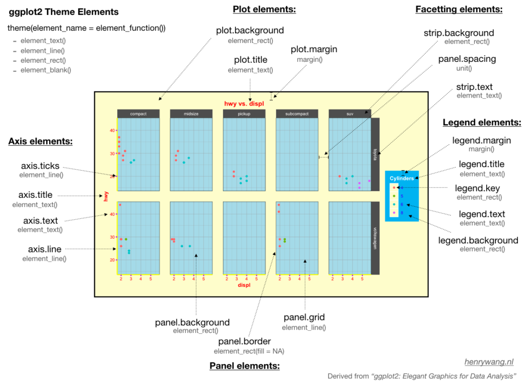
If you have trouble, as I do, remembering the various theme elements, this blog post from Henry Wang has a nice overview to help you.

Have any questions? Put them below and we will help you out!

You need to be signed-in to comment on this post. Login.

Matt Newman • May 21, 2024

I just learned something the hard way! A function doesn't seem to get updated if you tweak and rerun that code. Instead, I realized I need to restart my R session and create the updated function anew. Pretty nice looking custom theme, if I do say so myself!

theme_fugly <- function() {

theme_minimal() +
theme(axis.title = element_blank(),
      axis.text = element_text(color = "purple",
                               size = 25 ),
      legend.position = "none",
      panel.border = element_rect(color = "limegreen",
                                  linewidth = 5,
                                  fill = NA),
      plot.title = element_markdown(),
      plot.title.position = "plot",
      panel.grid.minor = element_blank(),
      panel.background = element_rect(fill = "navy"))
}

David Keyes Founder • May 21, 2024

Ha, nice theme!

But wait, your function didn't get updated when you reran the code? Did you highlight the full function and run it? Or just put your cursor on the theme_fugly <- function() { run and hit command/control (Mac/Windows) and enter? That should update your function.